A while back I was looking into treebanks (something that a future edition of CLM should probably spend more time on than the current one, which basically just points out that they exist). I created some small treebanks, trying out different parsers and manually correcting their output. In order to find errors in the parse, I used Yoichiro Hasebe’s great online tool RSyntaxTree – so named because it is written in Ruby, not, unfortunately, in R – to visualize the trees.
Then it struck me how great it would be if I could actually use R to draw the trees for me instead. I looked around for a package that would do this, and I don’t remember if I couldn’t find one or if I just didn’t like what I found. Anyway, I decided to come up with a way on my own – and I did, relying almost exclusively on existing packages. This post describes how.
First, I obviously did not want to write any code for drawing the trees, since there are plenty of packages that can do so in the context of cluster analyisis, network visualization etc. In the end, I settled on the ggraph package (CRAN) in combination with the igraph package (CRAN), but once you have seen how I coaxed them into drawing syntax trees, I’m sure you can adapt the strategy to other packages of your choice.
ggraph is a tool for network visualisation. In oder to get it to draw syntax trees, we have to turn our syntactic parse into a data structure that can be visualized as a network. Most obviously, this would be an edge list. If you are very patient, you can create an edge list from a parse manually, but instead, I therefore wrote an R function to convert a PTB parse to a data frame which, among other things, contains a column listing all nodes in the parse and a column listing their mothers.
I call this data fram synframe and the function ptb2synframe). You can download it from my github repository – feel free to modify or build on it in any way you want. The function takes a single argument: A PTB parse like the following:
(S (NP (DT The) (JJ happy) (JJ little) (NN dog)) (VP (VP (VBD ate) (NP (PDT all) (DT the) (NNS biscuits))
To turn such a parse into a synframe, you first import the function as follows (here, the command fetches the file from my github repository; if you have downloaded the script, replace the URL by your local path to the file):
source("https://raw.githubusercontent.com/astefanowitsch/various/main/ptb2synframe.R")
Now, run the ptb2synframe command in R:
ptb2synframe("(S (NP (DT The) (JJ happy) (JJ little) (NN dog)) (VP (VBD ate) (NP (PDT all) (DT the) (NNS bisquits))))") -> my.synframe
The resulting synframe looks like this:
   Index     Name        Node Level Terminal Mother
1      1        S         S-1     1        0   ROOT
2      2       NP        NP-2     2        0    S-1
3      3       DT        DT-3     3        0   NP-2
4      4      The       The-4     4        1   DT-3
5      5       JJ        JJ-5     3        0   NP-2
6      6    happy     happy-6     4        1   JJ-5
7      7       JJ        JJ-7     3        0   NP-2
8      8   little    little-8     4        1   JJ-7
9      9       NN        NN-9     3        0   NP-2
10    10      dog      dog-10     4        1   NN-9
11    11       VP       VP-11     2        0    S-1
12    12       VP       VP-12     3        0  VP-11
13    13      VBD      VBD-13     4        0  VP-12
14    14      ate      ate-14     5        1 VBD-13
15    15       NP       NP-15     4        0  VP-12
16    16      PDT      PDT-16     5        0  NP-15
17    17      all      all-17     6        1 PDT-16
18    18       DT       DT-18     5        0  NP-15
19    19      the      the-19     6        1  DT-18
20    20      NNS      NNS-20     5        0  NP-15
21    21 bisquits bisquits-21     6        1 NNS-20
As you can see, the first column is simply an index of the position of the node in the parse, the second column contains the node as it is present in the parse. The third column contains the nodes, combined with their index, mainly to make their names unique. The next column contains the level of nesting and the one after that contains the information whether or not the node is a terminal one (neither of these are needed here, but I feel they might come in handy for other purposes). Finally, the last column contains the mothers of the nodes in the third column.
In order to turn this into an edge list, we simply have to create a data frame containing just the Node and the Mother columns, renamed from and to respectively:
my.edgelist <- data.frame("from"=my.synframe$Mother,"to"=my.synframe$Node)
(Note that it would be easy to rewrite the ptb2synframe function in a way that creates the edge list directly, if you want to skip this step).
This is all that is needed to let igraph and ggraph work their magic!
Don’t forget to load the required libraries:
library(igraph)

library(ggraph)
Now, turn the edge list into an igraph, using the command graph_from_data_frame:
my.igraph <- graph_from_data_frame(my.edgelist)
Next, use ggraph to visualize the tree. ggraph is a powerful package that can draw all kinds of trees. To get a relatively standard-looking tree, try the following:
ggraph(my.igraph, layout = 'tree', circular = FALSE) +
    geom_edge_link() +
    geom_node_point(color="white",size=5) +
    geom_node_text(aes(label=name),size=3,nudge_y=-0.01) +
    theme_void()
This will yield something like this:
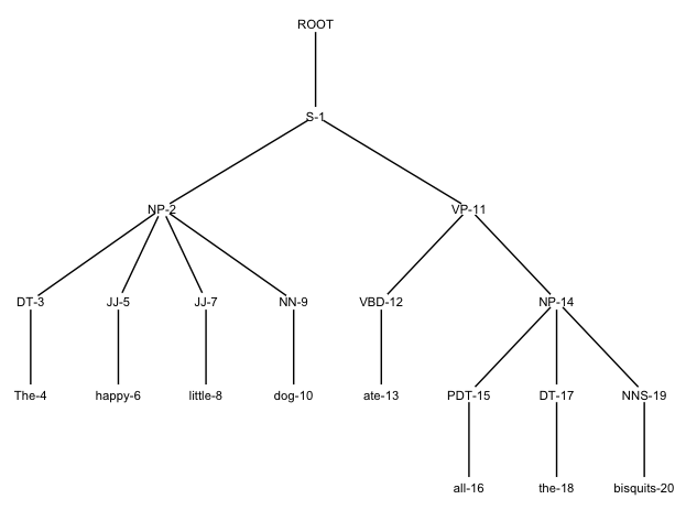
You can play around with the look of the tree by resizing the canvas, adjusting font size and color and nudging the labels upwards or downwards a bit by changing the value of nudge_y, until you like what you see.
Note that the node labels still show the indices. This may be useful if, like me, you want to use these trees to find and correct errors in the parse – they provide additional orientation. However, if you want to get rid of them, you can, by using the gsub function to remove them using a regular expression:
ggraph(my.igraph, layout = 'tree', circular = FALSE) +
    geom_edge_link() +
    geom_node_point(color="white",size=5) +
    geom_node_text(aes(label=gsub("(\\S+)- \\d+","\\1",names(my.igraph[1]))),size=3,nudge_y=-0.01) +
    theme_void()
This will draw the same tree as before, without the indices:

This was really all I wanted, so I could have stopped here. But by this time, it was three in the morning, and I was a bit lightheaded from sleep deprivation, so I decided I would no longer be bound by traditions concerning the visual representation of syntax trees. As mentioned above, ggraph can draw all kinds of trees – a nice overview is provided here. So I played with the package for a few hours, producing ever more creative trees. Here is a selection of not even the weirdest things I produced:
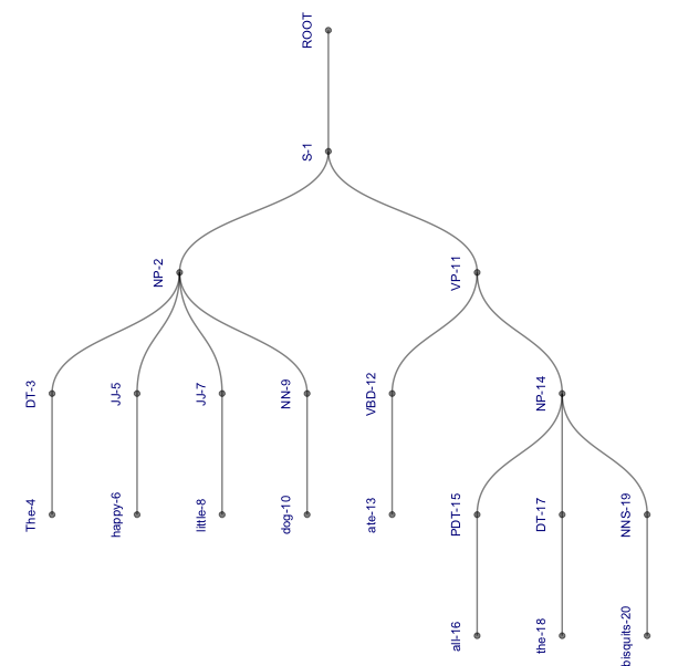
1. A fairly standard tree with lightblue branches and darkblue labels, which are displayed vertically next to their nodes (note that the colour attribute requires the British English spelling):
ggraph(my.igraph, layout = 'tree', circular = FALSE) +
    geom_edge_link(colour="lightblue") +
    geom_node_point(alpha=0.5) +
    geom_node_text(aes(label=name),size=3,angle=90,nudge_x=-0.25,color="darkblue") +
    theme_void()

2. The same tree turned sideways using the flipgraph command (see here for information about how to use this command):
flipgraph <- ggraph(my.igraph, layout = 'tree', circular = FALSE) +
    geom_edge_link(colour="lightblue") +
    geom_node_point(alpha=0.5) +
    geom_node_text(aes(label=name),size=3,angle=0,nudge_x=-0.3,color="darkblue") +
    theme_void()
flipgraph + scale_x_reverse() + scale_y_reverse() + coord_flip()

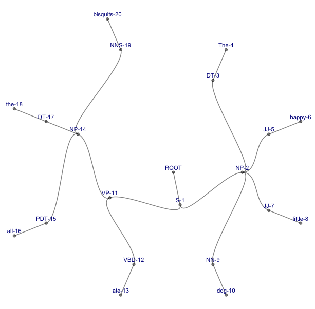
3. A strangely beautiful tree with curved branches and the labels appearing vertically next to their nodes – this instantly became my favorite representation:
ggraph(my.igraph, layout = 'tree', circular = FALSE) +
    geom_edge_diagonal(alpha=0.5) +
    geom_node_point(alpha=0.5) +
    geom_node_text(aes(label=name),size=3,angle=90,nudge_x=-0.25,color="darkblue") +
    theme_void()
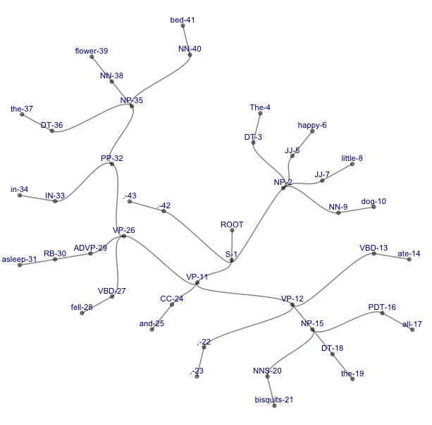
4. A circular tree with curved branches (pushing it beyond the beautiful into the domain of trippy):
ggraph(my.igraph, layout = 'tree', circular = TRUE) +
    geom_edge_diagonal(alpha=0.5) +
    geom_node_point(alpha=0.5) +
    geom_node_text(aes(label=name),size=3,nudge_y=0.03,color="darkblue") +
    theme_void()
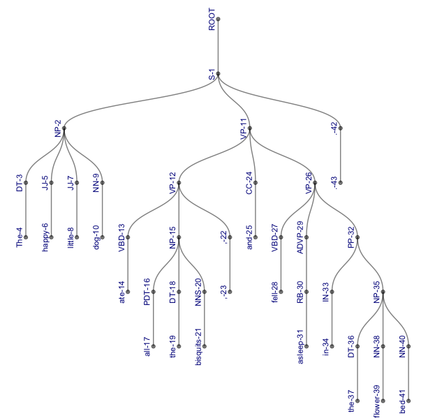
However, note that this representation might become useful with longer, more complex sentences, where it is more compact than our traditional representations (and even if it’s not, it is certainly more sciency-looking). Compare the following trees, both of which represent the parse (S (NP (DT The) (JJ happy) (JJ little) (NN dog)) (VP (VP (VBD ate) (NP (PDT all) (DT the) (NNS bisquits)) (, ,)) (CC and) (VP (VBD fell) (ADVP (RB asleep)) (PP (IN in) (NP (DT the) (NN flower) (NN bed))))) (. .)).
Thank you for reading, feedback is welcome!